Supplementary Work-In-Progress US Brands Signal Correlation Study
Contents
Supplementary Work-In-Progress US Brands Signal Correlation Study#
Similar to the work done on UK supermarkets, except in this case we don’t particularly care if the sales include eCommerce or not - because if we did that, we wouldn’t have many reference to showcase the power of this product.
# Configuration and import
import pandas as pd
import matplotlib.pyplot as plt
import seaborn as sns
from IPython.display import display

sns.set_style("darkgrid")
sns.set(rc={"figure.figsize": (15, 5)})

# Dataframe display util
def display_shrinked_dataframe(df_big):
    display(
        pd.concat(
            [df_big.select_dtypes(include="datetime").astype(str), df_big.select_dtypes(exclude="datetime")],
            axis=1,
        ).style.set_table_attributes('style="font-size: 8px"')
    )
df = pd.concat(
    [
        pd.read_parquet("./data/output/advance_auto_parts.parquet"),
        pd.read_parquet("./data/output/boot_barn.parquet"),
        pd.read_parquet("./data/output/walmart.parquet"),
        pd.read_parquet("./data/output/burlington_stores.parquet"),
        pd.read_parquet("./data/output/petco.parquet"),
    ],
    axis=1,
)
TARGETS = {}
SIGNALS = {}
# A small helper in evaluating correlation between two series
import scipy
import matplotlib.pyplot as plt
from sklearn.linear_model import LinearRegression
import numpy as np


def evaluate(signals, targets):
    signal_series = pd.Series(signals)
    target_series = pd.Series(targets)
    fig, ax = plt.subplots(1, 1, figsize=(15, 5))
    pearsonr, pval = scipy.stats.pearsonr(signal_series, target_series)

    ax.scatter(signal_series, target_series)
    ax.set_title(f"Pearson R: {round(pearsonr, 3)} - pval: {round(pval, 7)}")

    # LR to illustrate correlation, not used as prediction.
    linear_regression = LinearRegression()
    df_signal = pd.DataFrame({"signal": signal_series})
    linear_regression.fit(df_signal, target_series)
    xs = np.linspace(signal_series.min(), signal_series.max(), 10)
    ax.plot(xs, linear_regression.predict(pd.DataFrame({"signal": xs})), "r--")

    # Add some annotation
    for text, coor in (pd.concat([signal_series.rename("x"), target_series.rename("y")], axis=1)).iterrows():
        ax.annotate(text, (coor["x"], coor["y"]))

    plt.xlabel("Signal")
    plt.ylabel("Target (10-Q)")
# A small helper to extract signal sum to 10q dataframe
def extract_siganl_sum(df_10q, brand):
    for modifier in ['base', 'comp']:
        for ind, row in df_10q.iterrows():
            normalised_traffic = df[brand]
            normalised_traffic_filtered = normalised_traffic[
                (normalised_traffic.index >= row[f"{modifier}_start_date"])
                & (normalised_traffic.index <= row[f"{modifier}_end_date"])
            ]

            signal_len = len(normalised_traffic_filtered.index)
            target_len = (row[f"{modifier}_end_date"] - row[f"{modifier}_start_date"]).days + 1

            if abs(signal_len - target_len) > 0:
                raise RuntimeError()

            df_10q.loc[ind, f"{modifier}_summed_visit_duration_per_capita"] = normalised_traffic_filtered.sum()
# A small helper to read 10q dataframe and create the start dates in 10-Q dataframe
def read_10q(path):
    df_10q = pd.read_csv(path, parse_dates=["comp_end_date", "base_end_date"])

    if "comp_weeks" in df_10q.columns:
        print('creating start dates from weeks')
        df_10q["comp_start_date"] = df_10q["comp_end_date"] - pd.Timedelta("7 days") * df_10q["comp_weeks"]
        df_10q["base_start_date"] = df_10q["base_end_date"] - pd.Timedelta("7 days") * df_10q["base_weeks"]
    if "comp_months" in df_10q.columns:
        print('creating start dates from calendar months')
        with warnings.catch_warnings():
            df_10q["comp_start_date"] = df_10q["comp_end_date"] - df_10q['comp_months'].apply(pd.offsets.MonthBegin)
            df_10q["base_start_date"] = df_10q["base_end_date"] - df_10q['base_months'].apply(pd.offsets.MonthBegin)
    if "comp_modifier" in df_10q.columns:
        print("modifing net sales values by modifier")
        df_10q["comp_net_sales"] = df_10q["comp_net_sales"] * df_10q["comp_modifier"]
        df_10q["base_net_sales"] = df_10q["base_net_sales"] * df_10q["base_modifier"]
    if "comp_subtraction" in df_10q.columns:
        print("sutracting net sales values by indicated amount")
        df_10q["comp_net_sales"] = df_10q["comp_net_sales"] - df_10q["comp_subtraction"]
        df_10q["base_net_sales"] = df_10q["base_net_sales"] - df_10q["base_subtraction"]

    return df_10q
# A small helper to extract the signal and targets
def extract_signals_and_targets(df_10q, ticker):
    df_10q["target"] = TARGETS[ticker] = 100 * (
        (df_10q["comp_net_sales"] - df_10q["base_net_sales"]) / df_10q["base_net_sales"]
    )
    df_10q["signal"] = SIGNALS[ticker] = 100 * (
        (df_10q["comp_summed_visit_duration_per_capita"] - df_10q["base_summed_visit_duration_per_capita"])
        / df_10q["base_summed_visit_duration_per_capita"]
    )
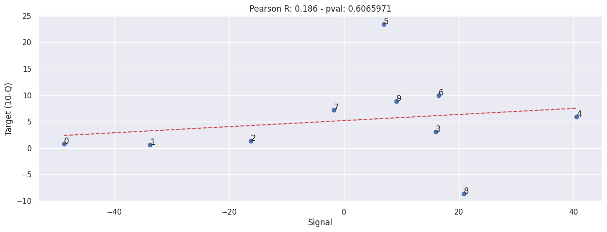
Advance Auto Part#
NOTE: This includes eCommerce sales!!
df_aap_10q = read_10q('./data/advance-auto-parts-10q.csv')
display_shrinked_dataframe(df_aap_10q)
creating start dates from weeks
| comp_end_date | base_end_date | comp_start_date | base_start_date | comp_weeks | base_weeks | comp_net_sales | base_net_sales | |
|---|---|---|---|---|---|---|---|---|
| 0 | 2022-10-08 | 2021-10-09 | 2022-07-16 | 2021-07-17 | 12 | 12 | 2641341 | 2621229 |
| 1 | 2022-07-16 | 2021-07-17 | 2022-04-23 | 2021-04-24 | 12 | 12 | 2665426 | 2649415 |
| 2 | 2022-04-23 | 2021-04-24 | 2022-01-01 | 2021-01-02 | 16 | 16 | 3374210 | 3330370 |
| 3 | 2021-10-09 | 2020-10-03 | 2021-07-17 | 2020-07-11 | 12 | 12 | 2621229 | 2541928 |
| 4 | 2021-07-17 | 2020-07-11 | 2021-04-24 | 2020-04-18 | 12 | 12 | 2649415 | 2501380 |
| 5 | 2021-04-24 | 2020-04-18 | 2021-01-02 | 2019-12-28 | 16 | 16 | 3330370 | 2697882 |
| 6 | 2020-10-03 | 2019-10-05 | 2020-07-11 | 2019-07-13 | 12 | 12 | 2541928 | 2312106 |
| 7 | 2020-07-11 | 2019-07-13 | 2020-04-18 | 2019-04-20 | 12 | 12 | 2501380 | 2332246 |
| 8 | 2020-04-18 | 2019-04-20 | 2020-01-25 | 2019-01-26 | 12 | 12 | 2697882 | 2952036 |
| 9 | 2022-01-01 | 2021-01-02 | 2021-01-02 | 2019-12-28 | 52 | 53 | 10997989 | 10106321 |
extract_siganl_sum(df_aap_10q, "advance_auto_parts")
extract_signals_and_targets(df_aap_10q, "AAP")
evaluate(SIGNALS['AAP'], TARGETS['AAP'])
display_shrinked_dataframe(df_aap_10q)
| comp_end_date | base_end_date | comp_start_date | base_start_date | comp_weeks | base_weeks | comp_net_sales | base_net_sales | base_summed_visit_duration_per_capita | comp_summed_visit_duration_per_capita | target | signal | |
|---|---|---|---|---|---|---|---|---|---|---|---|---|
| 0 | 2022-10-08 | 2021-10-09 | 2022-07-16 | 2021-07-17 | 12 | 12 | 2641341 | 2621229 | 1.555123 | 0.796264 | 0.767274 | -48.797354 |
| 1 | 2022-07-16 | 2021-07-17 | 2022-04-23 | 2021-04-24 | 12 | 12 | 2665426 | 2649415 | 1.644793 | 1.088787 | 0.604322 | -33.803998 |
| 2 | 2022-04-23 | 2021-04-24 | 2022-01-01 | 2021-01-02 | 16 | 16 | 3374210 | 3330370 | 2.149711 | 1.800348 | 1.316370 | -16.251635 |
| 3 | 2021-10-09 | 2020-10-03 | 2021-07-17 | 2020-07-11 | 12 | 12 | 2621229 | 2541928 | 1.340966 | 1.555123 | 3.119719 | 15.970371 |
| 4 | 2021-07-17 | 2020-07-11 | 2021-04-24 | 2020-04-18 | 12 | 12 | 2649415 | 2501380 | 1.170456 | 1.644793 | 5.918133 | 40.525805 |
| 5 | 2021-04-24 | 2020-04-18 | 2021-01-02 | 2019-12-28 | 16 | 16 | 3330370 | 2697882 | 2.010605 | 2.149711 | 23.443872 | 6.918622 |
| 6 | 2020-10-03 | 2019-10-05 | 2020-07-11 | 2019-07-13 | 12 | 12 | 2541928 | 2312106 | 1.151300 | 1.340966 | 9.939942 | 16.474117 |
| 7 | 2020-07-11 | 2019-07-13 | 2020-04-18 | 2019-04-20 | 12 | 12 | 2501380 | 2332246 | 1.192041 | 1.170456 | 7.251979 | -1.810734 |
| 8 | 2020-04-18 | 2019-04-20 | 2020-01-25 | 2019-01-26 | 12 | 12 | 2697882 | 2952036 | 1.165395 | 1.408802 | -8.609448 | 20.886207 |
| 9 | 2022-01-01 | 2021-01-02 | 2021-01-02 | 2019-12-28 | 52 | 53 | 10997989 | 10106321 | 6.116946 | 6.677417 | 8.822874 | 9.162608 |
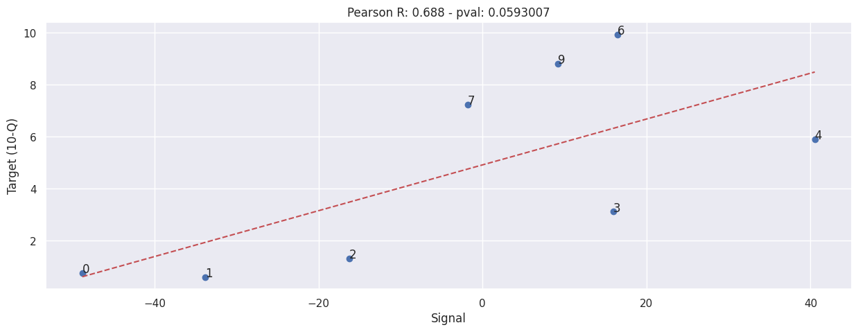
Aside - Remove clear outliers.#
Row 5 and row 8 are clearly outliers, this indicates exceptionally bad sales in the quarter ended 2020-04-18.
There is no clear explanation in the 10-Qs.
This is post-hoc analysis, take this with a grain of sale.
evaluate(SIGNALS["AAP"].drop([5, 8]), TARGETS["AAP"].drop([5,8]))
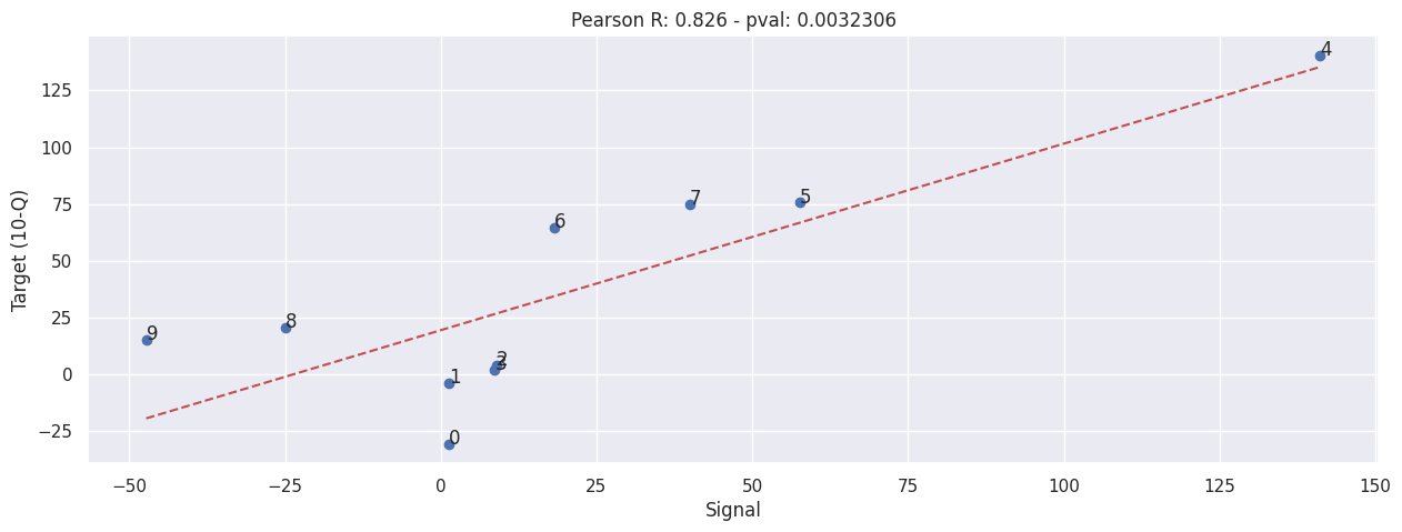
Boot Barn#
With eCommerce net sales removed - as the figures are included in the 10-Qs.
df_boot_10q = read_10q('./data/boot-barn-10q.csv')
display_shrinked_dataframe(df_boot_10q)
creating start dates from weeks
modifing net sales values by modifier
| comp_end_date | base_end_date | comp_start_date | base_start_date | comp_weeks | base_weeks | comp_net_sales | base_net_sales | comp_modifier | base_modifier | |
|---|---|---|---|---|---|---|---|---|---|---|
| 0 | 2020-06-27 | 2019-06-29 | 2020-03-28 | 2019-03-30 | 13 | 13 | 110824.500000 | 159759.620000 | 0.750000 | 0.860000 |
| 1 | 2020-09-26 | 2019-09-28 | 2020-06-27 | 2019-06-29 | 13 | 13 | 153147.450000 | 159105.550000 | 0.830000 | 0.850000 |
| 2 | 2020-12-26 | 2019-12-28 | 2020-09-26 | 2019-09-28 | 13 | 13 | 241870.400000 | 232877.540000 | 0.800000 | 0.820000 |
| 3 | 2021-03-27 | 2020-03-28 | 2020-03-28 | 2019-03-30 | 52 | 52 | 723727.710000 | 710283.000000 | 0.810000 | 0.840000 |
| 4 | 2021-06-26 | 2020-06-27 | 2021-03-27 | 2020-03-28 | 13 | 13 | 266504.490000 | 110824.500000 | 0.870000 | 0.750000 |
| 5 | 2021-09-25 | 2020-09-26 | 2021-06-26 | 2020-06-27 | 13 | 13 | 268936.620000 | 153147.450000 | 0.860000 | 0.830000 |
| 6 | 2021-12-25 | 2020-12-26 | 2021-09-25 | 2020-09-26 | 13 | 13 | 398441.280000 | 241870.400000 | 0.820000 | 0.800000 |
| 7 | 2022-03-26 | 2021-03-27 | 2021-03-27 | 2020-03-28 | 52 | 52 | 1265017.600000 | 723727.710000 | 0.850000 | 0.810000 |
| 8 | 2022-06-25 | 2021-06-26 | 2022-03-26 | 2021-03-27 | 13 | 13 | 321953.280000 | 266504.490000 | 0.880000 | 0.870000 |
| 9 | 2022-09-24 | 2021-09-25 | 2022-06-25 | 2021-06-26 | 13 | 13 | 309359.600000 | 268936.620000 | 0.880000 | 0.860000 |
extract_siganl_sum(df_boot_10q, "boot_barn")
extract_signals_and_targets(df_boot_10q, "BOOT")
evaluate(SIGNALS['BOOT'], TARGETS['BOOT'])
display_shrinked_dataframe(df_boot_10q)
| comp_end_date | base_end_date | comp_start_date | base_start_date | comp_weeks | base_weeks | comp_net_sales | base_net_sales | comp_modifier | base_modifier | base_summed_visit_duration_per_capita | comp_summed_visit_duration_per_capita | target | signal | |
|---|---|---|---|---|---|---|---|---|---|---|---|---|---|---|
| 0 | 2020-06-27 | 2019-06-29 | 2020-03-28 | 2019-03-30 | 13 | 13 | 110824.500000 | 159759.620000 | 0.750000 | 0.860000 | 0.122293 | 0.123824 | -30.630468 | 1.251131 |
| 1 | 2020-09-26 | 2019-09-28 | 2020-06-27 | 2019-06-29 | 13 | 13 | 153147.450000 | 159105.550000 | 0.830000 | 0.850000 | 0.153366 | 0.155375 | -3.744747 | 1.309601 |
| 2 | 2020-12-26 | 2019-12-28 | 2020-09-26 | 2019-09-28 | 13 | 13 | 241870.400000 | 232877.540000 | 0.800000 | 0.820000 | 0.223805 | 0.243911 | 3.861626 | 8.983932 |
| 3 | 2021-03-27 | 2020-03-28 | 2020-03-28 | 2019-03-30 | 52 | 52 | 723727.710000 | 710283.000000 | 0.810000 | 0.840000 | 0.729244 | 0.792602 | 1.892867 | 8.688159 |
| 4 | 2021-06-26 | 2020-06-27 | 2021-03-27 | 2020-03-28 | 13 | 13 | 266504.490000 | 110824.500000 | 0.870000 | 0.750000 | 0.123824 | 0.298612 | 140.474345 | 141.159248 |
| 5 | 2021-09-25 | 2020-09-26 | 2021-06-26 | 2020-06-27 | 13 | 13 | 268936.620000 | 153147.450000 | 0.860000 | 0.830000 | 0.155375 | 0.244802 | 75.606332 | 57.555348 |
| 6 | 2021-12-25 | 2020-12-26 | 2021-09-25 | 2020-09-26 | 13 | 13 | 398441.280000 | 241870.400000 | 0.820000 | 0.800000 | 0.243911 | 0.288428 | 64.733378 | 18.251134 |
| 7 | 2022-03-26 | 2021-03-27 | 2021-03-27 | 2020-03-28 | 52 | 52 | 1265017.600000 | 723727.710000 | 0.850000 | 0.810000 | 0.792602 | 1.109396 | 74.791926 | 39.968932 |
| 8 | 2022-06-25 | 2021-06-26 | 2022-03-26 | 2021-03-27 | 13 | 13 | 321953.280000 | 266504.490000 | 0.880000 | 0.870000 | 0.298612 | 0.224125 | 20.805950 | -24.944393 |
| 9 | 2022-09-24 | 2021-09-25 | 2022-06-25 | 2021-06-26 | 13 | 13 | 309359.600000 | 268936.620000 | 0.880000 | 0.860000 | 0.244802 | 0.129066 | 15.030672 | -47.277176 |
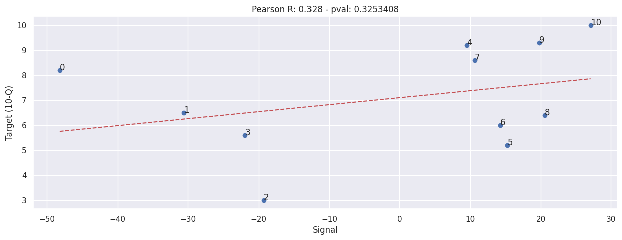
Walmart#
NOTE: This includes eCommerce sales!!
We use the comp sales figures instead of raw net sales because net sales includes fuel sales, and that is extremely volatile according to Walmart’s own report.
df_wmt_10q = pd.read_csv("./data/walmart-10q-comp.csv", parse_dates=["base_end_date", "comp_end_date"])
df_wmt_10q["base_start_date"] = df_wmt_10q["base_end_date"] - (pd.Timedelta("7 days") * df_wmt_10q["weeks"])
df_wmt_10q["comp_start_date"] = df_wmt_10q["comp_end_date"] - (pd.Timedelta("7 days") * df_wmt_10q["weeks"])
display_shrinked_dataframe(df_wmt_10q)
| comp_end_date | base_end_date | base_start_date | comp_start_date | weeks | comp_sales_pct | |
|---|---|---|---|---|---|---|
| 0 | 2022-10-28 | 2021-10-29 | 2021-07-30 | 2022-07-29 | 13 | 8.200000 |
| 1 | 2022-07-29 | 2021-07-30 | 2021-04-30 | 2022-04-29 | 13 | 6.500000 |
| 2 | 2022-04-29 | 2021-04-30 | 2021-01-29 | 2022-01-28 | 13 | 3.000000 |
| 3 | 2022-01-28 | 2021-01-29 | 2020-10-30 | 2021-10-29 | 13 | 5.600000 |
| 4 | 2021-10-29 | 2020-10-30 | 2020-07-31 | 2021-07-30 | 13 | 9.200000 |
| 5 | 2021-07-30 | 2020-07-31 | 2020-05-01 | 2021-04-30 | 13 | 5.200000 |
| 6 | 2021-04-30 | 2020-05-01 | 2020-01-31 | 2021-01-29 | 13 | 6.000000 |
| 7 | 2021-01-29 | 2020-01-31 | 2019-11-01 | 2020-10-30 | 13 | 8.600000 |
| 8 | 2020-10-30 | 2019-10-25 | 2019-07-26 | 2020-07-31 | 13 | 6.400000 |
| 9 | 2020-07-31 | 2019-07-26 | 2019-04-26 | 2020-05-01 | 13 | 9.300000 |
| 10 | 2020-05-01 | 2019-04-26 | 2019-01-25 | 2020-01-31 | 13 | 10.000000 |
extract_siganl_sum(df_wmt_10q, "walmart")
TARGETS["WMT"] = df_wmt_10q["target"] = df_wmt_10q["comp_sales_pct"]

SIGNALS["WMT"] = df_wmt_10q["signal"] = 100 * (
    (
        df_wmt_10q["comp_summed_visit_duration_per_capita"]
        - df_wmt_10q["base_summed_visit_duration_per_capita"]
    )
    / df_wmt_10q["base_summed_visit_duration_per_capita"]
)
evaluate(SIGNALS['WMT'], TARGETS['WMT'])
display_shrinked_dataframe(df_wmt_10q)
| comp_end_date | base_end_date | base_start_date | comp_start_date | weeks | comp_sales_pct | base_summed_visit_duration_per_capita | comp_summed_visit_duration_per_capita | target | signal | |
|---|---|---|---|---|---|---|---|---|---|---|
| 0 | 2022-10-28 | 2021-10-29 | 2021-07-30 | 2022-07-29 | 13 | 8.200000 | 75.974168 | 39.361808 | 8.200000 | -48.190538 |
| 1 | 2022-07-29 | 2021-07-30 | 2021-04-30 | 2022-04-29 | 13 | 6.500000 | 86.744224 | 60.230678 | 6.500000 | -30.565201 |
| 2 | 2022-04-29 | 2021-04-30 | 2021-01-29 | 2022-01-28 | 13 | 3.000000 | 86.644477 | 69.944291 | 3.000000 | -19.274380 |
| 3 | 2022-01-28 | 2021-01-29 | 2020-10-30 | 2021-10-29 | 13 | 5.600000 | 91.421580 | 71.363799 | 5.600000 | -21.939875 |
| 4 | 2021-10-29 | 2020-10-30 | 2020-07-31 | 2021-07-30 | 13 | 9.200000 | 69.353002 | 75.974168 | 9.200000 | 9.547050 |
| 5 | 2021-07-30 | 2020-07-31 | 2020-05-01 | 2021-04-30 | 13 | 5.200000 | 75.222506 | 86.744224 | 5.200000 | 15.316849 |
| 6 | 2021-04-30 | 2020-05-01 | 2020-01-31 | 2021-01-29 | 13 | 6.000000 | 75.817399 | 86.644477 | 6.000000 | 14.280465 |
| 7 | 2021-01-29 | 2020-01-31 | 2019-11-01 | 2020-10-30 | 13 | 8.600000 | 82.640186 | 91.421580 | 8.600000 | 10.626058 |
| 8 | 2020-10-30 | 2019-10-25 | 2019-07-26 | 2020-07-31 | 13 | 6.400000 | 57.514451 | 69.353002 | 6.400000 | 20.583611 |
| 9 | 2020-07-31 | 2019-07-26 | 2019-04-26 | 2020-05-01 | 13 | 9.300000 | 62.802444 | 75.222506 | 9.300000 | 19.776400 |
| 10 | 2020-05-01 | 2019-04-26 | 2019-01-25 | 2020-01-31 | 13 | 10.000000 | 59.655455 | 75.817399 | 10.000000 | 27.092149 |
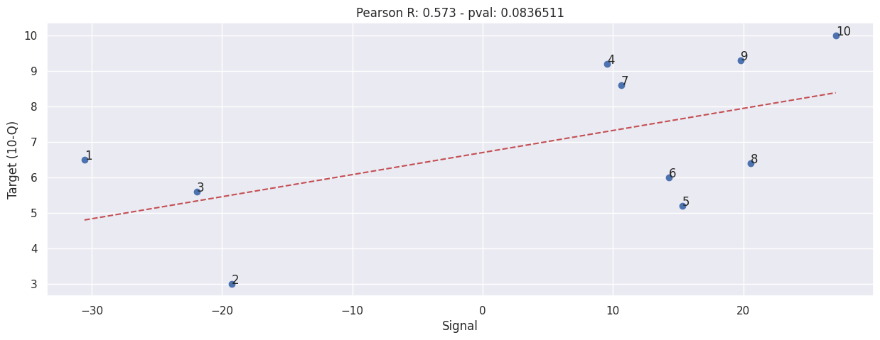
Aside: Without outlier#
Just an experiement to see if we remove the 0th row, what happens.
Take this with a grain of salt!
evaluate(SIGNALS['WMT'].drop([0]), TARGETS['WMT'].drop([0]))
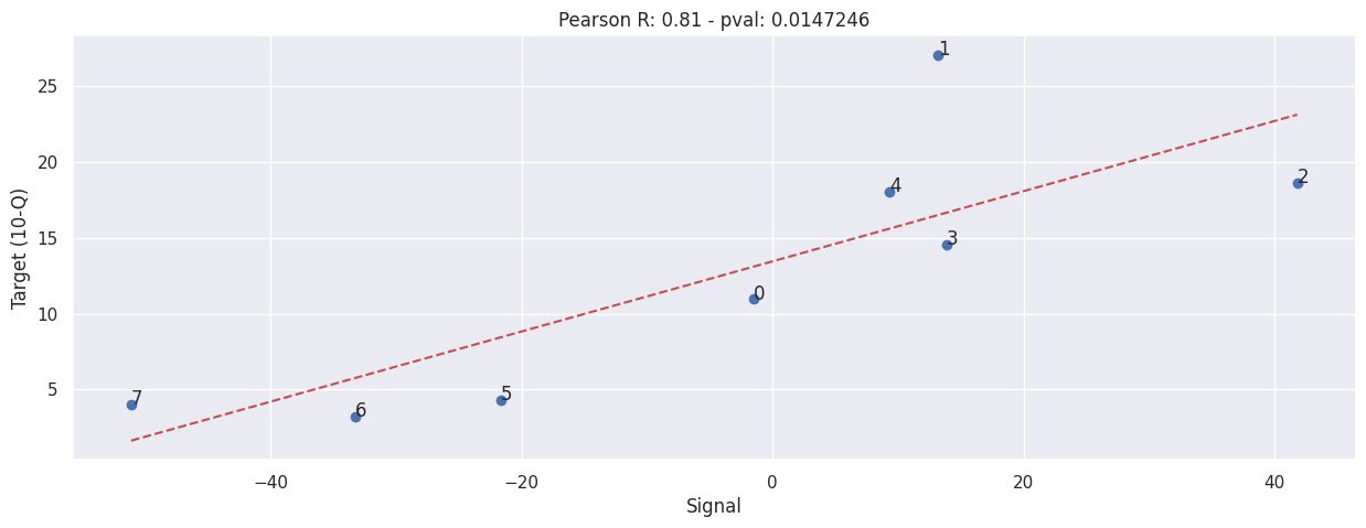
Petco#
NOTE: This includes eCommerce sales!!
df_woof_10q = read_10q('./data/petco-10q.csv')
display_shrinked_dataframe(df_woof_10q)
creating start dates from weeks
| comp_end_date | base_end_date | comp_start_date | base_start_date | comp_weeks | base_weeks | comp_net_sales | base_net_sales | |
|---|---|---|---|---|---|---|---|---|
| 0 | 2021-01-30 | 2020-02-01 | 2020-02-01 | 2019-02-02 | 52 | 52 | 4920202 | 4434514 |
| 1 | 2021-05-01 | 2020-05-02 | 2021-01-30 | 2020-02-01 | 13 | 13 | 1414994 | 1113521 |
| 2 | 2021-07-31 | 2020-08-01 | 2021-05-01 | 2020-05-02 | 13 | 13 | 1434534 | 1208971 |
| 3 | 2021-10-30 | 2020-10-31 | 2021-07-31 | 2020-08-01 | 13 | 13 | 1443264 | 1259997 |
| 4 | 2022-01-29 | 2021-01-30 | 2021-01-30 | 2020-02-01 | 52 | 52 | 5807149 | 4920202 |
| 5 | 2022-04-30 | 2021-05-01 | 2022-01-29 | 2021-01-30 | 13 | 13 | 1475991 | 1414994 |
| 6 | 2022-07-30 | 2021-07-31 | 2022-04-30 | 2021-05-01 | 13 | 13 | 1480797 | 1434534 |
| 7 | 2022-10-29 | 2021-10-30 | 2022-07-30 | 2021-07-31 | 13 | 13 | 1501220 | 1443264 |
extract_siganl_sum(df_10q=df_woof_10q, brand="petco")
extract_signals_and_targets(df_woof_10q, "WOOF")
evaluate(SIGNALS["WOOF"], TARGETS["WOOF"])
display_shrinked_dataframe(df_woof_10q)
| comp_end_date | base_end_date | comp_start_date | base_start_date | comp_weeks | base_weeks | comp_net_sales | base_net_sales | base_summed_visit_duration_per_capita | comp_summed_visit_duration_per_capita | target | signal | |
|---|---|---|---|---|---|---|---|---|---|---|---|---|
| 0 | 2021-01-30 | 2020-02-01 | 2020-02-01 | 2019-02-02 | 52 | 52 | 4920202 | 4434514 | 6.594067 | 6.493723 | 10.952452 | -1.521740 |
| 1 | 2021-05-01 | 2020-05-02 | 2021-01-30 | 2020-02-01 | 13 | 13 | 1414994 | 1113521 | 1.736050 | 1.964243 | 27.073850 | 13.144354 |
| 2 | 2021-07-31 | 2020-08-01 | 2021-05-01 | 2020-05-02 | 13 | 13 | 1434534 | 1208971 | 1.373632 | 1.947683 | 18.657437 | 41.790801 |
| 3 | 2021-10-30 | 2020-10-31 | 2021-07-31 | 2020-08-01 | 13 | 13 | 1443264 | 1259997 | 1.526434 | 1.737888 | 14.545035 | 13.852821 |
| 4 | 2022-01-29 | 2021-01-30 | 2021-01-30 | 2020-02-01 | 52 | 52 | 5807149 | 4920202 | 6.493723 | 7.097429 | 18.026638 | 9.296771 |
| 5 | 2022-04-30 | 2021-05-01 | 2022-01-29 | 2021-01-30 | 13 | 13 | 1475991 | 1414994 | 1.964243 | 1.538701 | 4.310760 | -21.664438 |
| 6 | 2022-07-30 | 2021-07-31 | 2022-04-30 | 2021-05-01 | 13 | 13 | 1480797 | 1434534 | 1.947683 | 1.299647 | 3.224950 | -33.272134 |
| 7 | 2022-10-29 | 2021-10-30 | 2022-07-30 | 2021-07-31 | 13 | 13 | 1501220 | 1443264 | 1.737888 | 0.849929 | 4.015620 | -51.094171 |
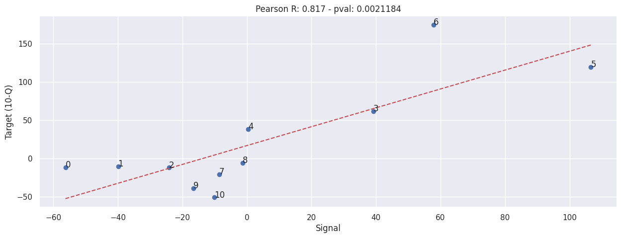
Burlington Stores#
NOTE: This includes eCommerce sales!!
df_burl_10q = read_10q('./data/burlington-stores-10q.csv')
display_shrinked_dataframe(df_burl_10q)
creating start dates from weeks
| comp_end_date | base_end_date | comp_start_date | base_start_date | comp_weeks | base_weeks | comp_net_sales | base_net_sales | |
|---|---|---|---|---|---|---|---|---|
| 0 | 2022-10-29 | 2021-10-30 | 2022-07-30 | 2021-07-31 | 13 | 13 | 2035927 | 2299610 |
| 1 | 2022-07-30 | 2021-07-31 | 2022-04-30 | 2021-05-01 | 13 | 13 | 1983889 | 2212812 |
| 2 | 2022-04-30 | 2021-05-01 | 2022-01-29 | 2021-01-30 | 13 | 13 | 1925643 | 2190667 |
| 3 | 2022-01-29 | 2021-01-30 | 2021-01-30 | 2020-02-01 | 52 | 52 | 9306549 | 5751541 |
| 4 | 2021-10-30 | 2021-10-31 | 2021-07-31 | 2021-08-01 | 13 | 13 | 2299610 | 1664728 |
| 5 | 2021-07-31 | 2020-08-01 | 2021-05-01 | 2020-05-02 | 13 | 13 | 2212812 | 1009882 |
| 6 | 2021-05-01 | 2020-05-02 | 2021-01-30 | 2020-02-01 | 13 | 13 | 2190667 | 797996 |
| 7 | 2021-01-30 | 2020-02-01 | 2020-02-01 | 2019-02-02 | 52 | 52 | 5751541 | 7261243 |
| 8 | 2020-10-31 | 2019-11-02 | 2020-08-01 | 2019-08-03 | 13 | 13 | 1664728 | 1774949 |
| 9 | 2020-08-01 | 2019-08-03 | 2020-05-02 | 2019-05-04 | 13 | 13 | 1009882 | 1656363 |
| 10 | 2020-05-02 | 2019-05-04 | 2020-02-01 | 2019-02-02 | 13 | 13 | 797996 | 1628547 |
extract_siganl_sum(df_10q=df_burl_10q, brand="burlington_stores")
extract_signals_and_targets(df_10q=df_burl_10q, ticker="BURL")
evaluate(SIGNALS["BURL"], TARGETS["BURL"])
display_shrinked_dataframe(df_burl_10q)
| comp_end_date | base_end_date | comp_start_date | base_start_date | comp_weeks | base_weeks | comp_net_sales | base_net_sales | base_summed_visit_duration_per_capita | comp_summed_visit_duration_per_capita | target | signal | |
|---|---|---|---|---|---|---|---|---|---|---|---|---|
| 0 | 2022-10-29 | 2021-10-30 | 2022-07-30 | 2021-07-31 | 13 | 13 | 2035927 | 2299610 | 2.559946 | 1.119996 | -11.466423 | -56.249237 |
| 1 | 2022-07-30 | 2021-07-31 | 2022-04-30 | 2021-05-01 | 13 | 13 | 1983889 | 2212812 | 2.736310 | 1.644039 | -10.345343 | -39.917658 |
| 2 | 2022-04-30 | 2021-05-01 | 2022-01-29 | 2021-01-30 | 13 | 13 | 1925643 | 2190667 | 2.605419 | 1.976573 | -12.097868 | -24.136077 |
| 3 | 2022-01-29 | 2021-01-30 | 2021-01-30 | 2020-02-01 | 52 | 52 | 9306549 | 5751541 | 7.338445 | 10.212191 | 61.809661 | 39.160148 |
| 4 | 2021-10-30 | 2021-10-31 | 2021-07-31 | 2021-08-01 | 13 | 13 | 2299610 | 1664728 | 2.550870 | 2.559946 | 38.137281 | 0.355837 |
| 5 | 2021-07-31 | 2020-08-01 | 2021-05-01 | 2020-05-02 | 13 | 13 | 2212812 | 1009882 | 1.324480 | 2.736310 | 119.115897 | 106.595120 |
| 6 | 2021-05-01 | 2020-05-02 | 2021-01-30 | 2020-02-01 | 13 | 13 | 2190667 | 797996 | 1.650779 | 2.605419 | 174.521050 | 57.829702 |
| 7 | 2021-01-30 | 2020-02-01 | 2020-02-01 | 2019-02-02 | 52 | 52 | 5751541 | 7261243 | 8.029907 | 7.338445 | -20.791234 | -8.611081 |
| 8 | 2020-10-31 | 2019-11-02 | 2020-08-01 | 2019-08-03 | 13 | 13 | 1664728 | 1774949 | 1.641189 | 1.619570 | -6.209812 | -1.317292 |
| 9 | 2020-08-01 | 2019-08-03 | 2020-05-02 | 2019-05-04 | 13 | 13 | 1009882 | 1656363 | 1.587068 | 1.324480 | -39.030152 | -16.545488 |
| 10 | 2020-05-02 | 2019-05-04 | 2020-02-01 | 2019-02-02 | 13 | 13 | 797996 | 1628547 | 1.836885 | 1.650779 | -50.999511 | -10.131635 |
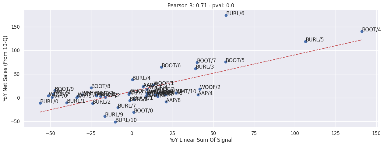
Overall#
This doesn’t incldue any removal of outliers at all.
evaluate(
    pd.concat([value.set_axis(value.index.map(lambda x: f"{key}/{x}")) for key, value in SIGNALS.items()]),
    pd.concat([value.set_axis(value.index.map(lambda x: f"{key}/{x}")) for key, value in TARGETS.items()]),
)
plt.xlabel("YoY Linear Sum Of Signal")
plt.ylabel("YoY Net Sales (From 10-Q)")
Text(0, 0.5, 'YoY Net Sales (From 10-Q)')