Consumer Bevahiour Analysis

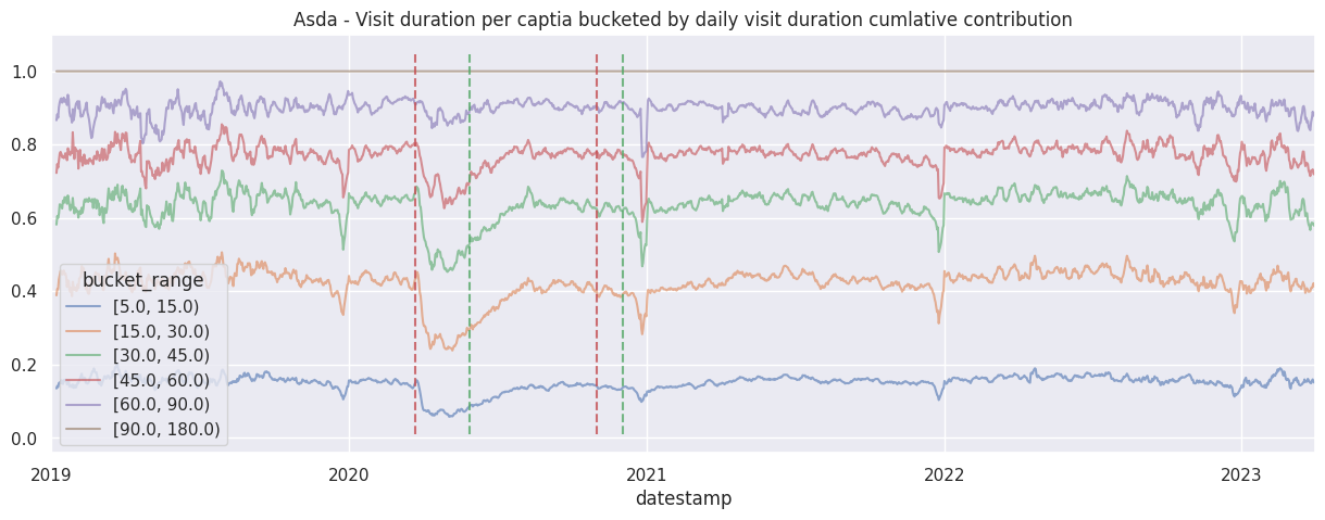
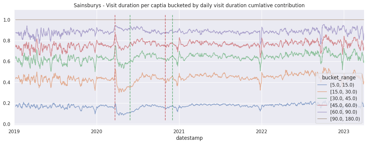
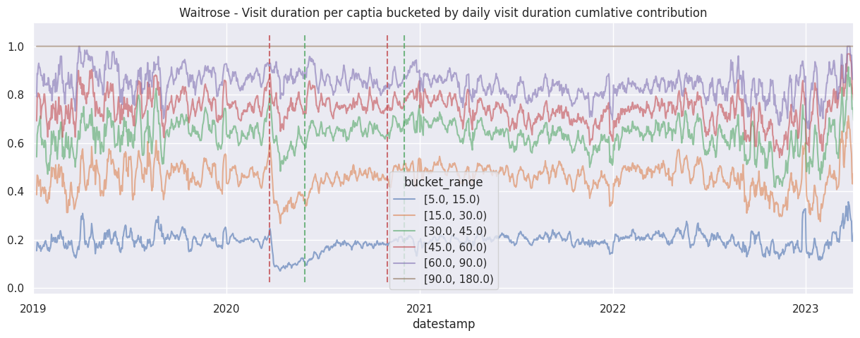
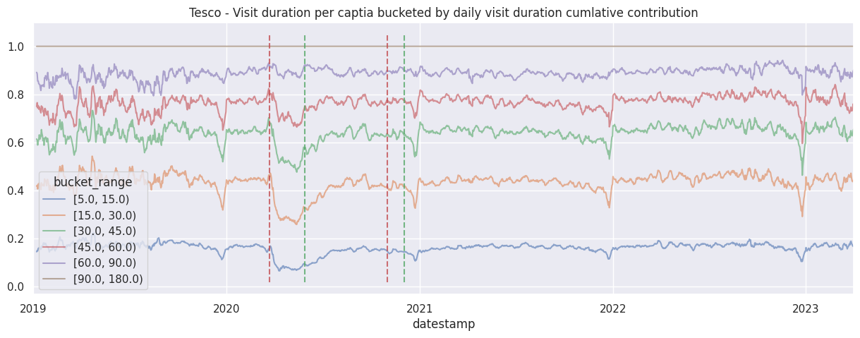
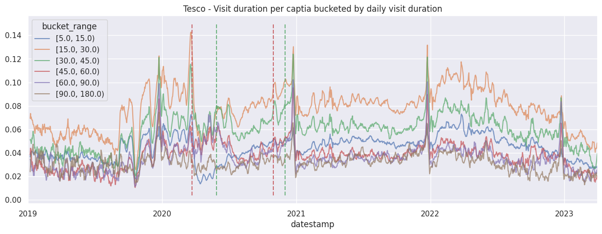
In this section we will perform some simple analysis on the bucketed signal, more specifically investigating how long do people spend in large supermarkets.

Even before looking at the data, we already suspect there will be drastic changes in behaviour near covid-19 lockdown periods based on anecdotal experience, these periods are of particular interest to us as it showcase how our data relates to the real world.

# Configuration and import
import constants
import datetime
import pandas as pd
import matplotlib.pyplot as plt
import seaborn as sns
from IPython.display import display

sns.set_style("darkgrid")
sns.set(rc={"figure.figsize": (15, 5)})

ALL_BUCKETS = range(1, len(constants.DWELL_BUCKETS))

# Read genereated signals
df = pd.concat(
    [
        pd.read_parquet("./data/output/asda-bucketed-daily.parquet"),
        pd.read_parquet("./data/output/sainsburys-bucketed-daily.parquet"),
        pd.read_parquet("./data/output/waitrose-bucketed-daily.parquet"),
        pd.read_parquet("./data/output/tesco-bucketed-daily.parquet"),
        pd.read_parquet("./data/output/morrison-bucketed-daily.parquet"),
    ],
    axis=1,
).reset_index()

# Convert the RANGE_BUCKET return value to actual ranges for reporting purposes.
PADDED_BUCKETS = [-float('inf'), *constants.DWELL_BUCKETS, float('inf')]
RANGES = pd.IntervalIndex.from_tuples(list(zip(PADDED_BUCKETS[:-1], PADDED_BUCKETS[1:])), closed='left')
RANGES_MAP = {
    bucket: RANGES[bucket]
    for bucket in ALL_BUCKETS
}

df["bucket_range"] = df["bucket"].map(RANGES_MAP)
df = df.dropna().drop(["bucket"], axis=1).copy()

# Stack the dataframe correctly for easier manipulation
df_stacked = df.set_index(["datestamp", "bucket_range"]).T.stack(level=1).T
# Grab all the brands
brands = df_stacked.columns.get_level_values(level=0).unique()

# Some plot helpers
def add_lockdown_lines(ax):
    ylim = ax.get_ylim()
    ax.vlines(
        [
            datetime.datetime(2020, 3, 23),
            datetime.datetime(2020, 10, 31),
        ],
        *ylim,
        "r",
        "--",
        alpha=0.8,
    )

    ax.vlines(
        [
            datetime.datetime(2020, 5, 28),
            datetime.datetime(2020, 12, 2),
        ],
        *ylim,
        "g",
        "--",
        alpha=0.8,
    )

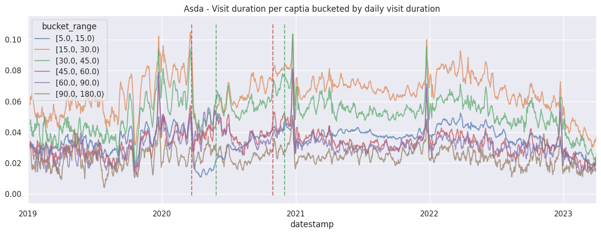
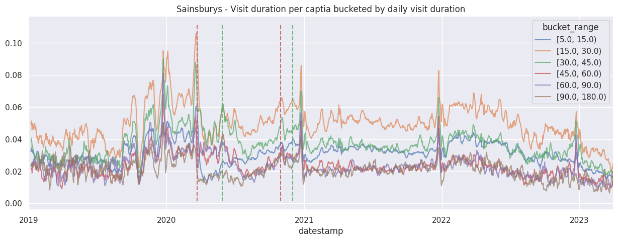
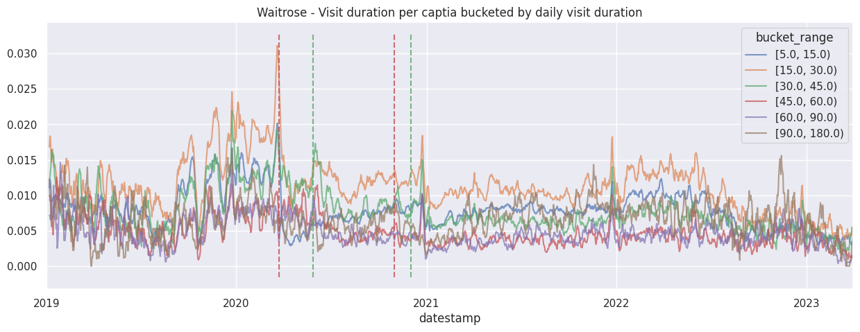
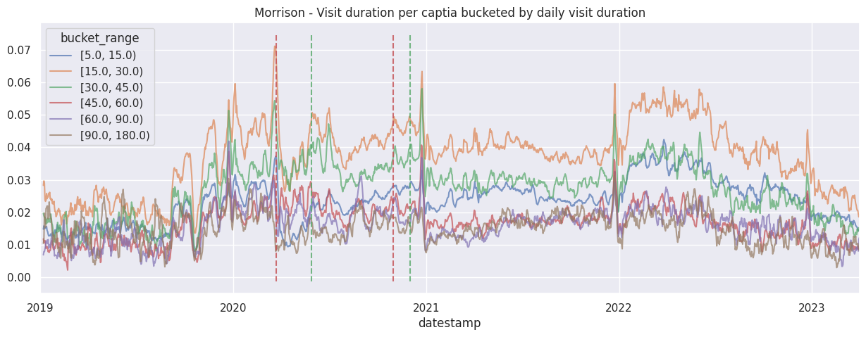
Examine the bucketed visit duration per brand by itself

for brand in brands:
    df_brand = df_stacked[brand]
    df_brand.rolling(7).mean().plot(alpha=0.7)
    ax = plt.gca()
    ax.set_title(f"{brand.title()} - Visit duration per captia bucketed by daily visit duration")
    add_lockdown_lines(ax)

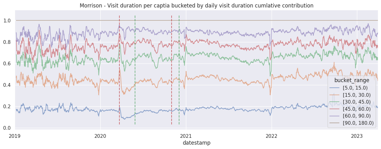
Examine the cumulative contribution bucketed visit duration per brand

for brand in brands:
    df_brand = df_stacked[brand]
    df_brand.div(df_brand.sum(axis=1), axis=0).cumsum(axis=1).rolling(7).mean().plot(alpha=0.6)
    ax = plt.gca()
    ax.set_title(f"{brand.title()} - Visit duration per captia bucketed by daily visit duration cumlative contribution")
    add_lockdown_lines(ax)