Bucketed Signal Correlation Study (Individual Visits)

In this section we will repeat the signal correlation study done before, with an important distinction that we will be correlating different subset of visit per captia separately, the bucket is determined by the length of the individual visits.

All caveats and notes from previous study applies here. See: Previous Study.

# Configuration and import
import constants
import pandas as pd
import matplotlib.pyplot as plt
import seaborn as sns
from IPython.display import display

sns.set_style("darkgrid")
sns.set(rc={"figure.figsize": (15, 5)})

# Dataframe display util
def display_shrinked_dataframe(df_big):
    display(
        pd.concat(
            [df_big.select_dtypes(include="datetime").astype(str), df_big.select_dtypes(exclude="datetime")],
            axis=1,
        ).style.set_table_attributes('style="font-size: 8px"')
    )
    
ALL_BUCKETS = range(1, len(constants.DWELL_BUCKETS))

# Read genereated signals
df = pd.concat(
    [
        pd.read_parquet("./data/output/asda-bucketed-individual.parquet"),
        pd.read_parquet("./data/output/sainsburys-bucketed-individual.parquet"),
        pd.read_parquet("./data/output/waitrose-bucketed-individual.parquet"),
        pd.read_parquet("./data/output/tesco-bucketed-individual.parquet"),
        pd.read_parquet("./data/output/morrison-bucketed-individual.parquet"),
    ],
    axis=1,
).unstack(level=-1)

TARGETS = {}
SIGNALS = {}

# A small helper in evaluating correlation between two series
import scipy
import matplotlib.pyplot as plt
from sklearn.linear_model import LinearRegression
import numpy as np


def evaluate(signals, targets, title_suffix):
    signal_series = pd.Series(signals)
    target_series = pd.Series(targets)
    fig, ax = plt.subplots(1, 1, figsize=(15, 5))
    pearsonr, pval = scipy.stats.pearsonr(signal_series, target_series)

    ax.scatter(signal_series, target_series)
    ax.set_title(f"Pearson R: {round(pearsonr, 3)} - pval: {round(pval, 3)} - {title_suffix}")

    # LR to illustrate correlation, not used as prediction.
    linear_regression = LinearRegression()
    df_signal = pd.DataFrame({"signal": signal_series})
    linear_regression.fit(df_signal, target_series)
    xs = np.linspace(signal_series.min(), signal_series.max(), 10)
    ax.plot(xs, linear_regression.predict(pd.DataFrame({"signal": xs})), "r--")

    # Add some annotation
    for text, coor in (pd.concat([signal_series.rename("x"), target_series.rename("y")], axis=1)).iterrows():
        ax.annotate(text, (coor["x"], coor["y"]))

    plt.xlabel("Signal")
    plt.ylabel("Target (10-Q)")

# A small helper to extract signal sum to 10q dataframe
def extract_siganl_sum(df_10q, brand):
    for modifier in ["base", "comp"]:
        for ind, row in df_10q.iterrows():
            for bucket in ALL_BUCKETS:
                normalised_traffic = df[brand, bucket]
                normalised_traffic_filtered = normalised_traffic[
                    (normalised_traffic.index >= row[f"{modifier}_start_date"])
                    & (normalised_traffic.index <= row[f"{modifier}_end_date"])
                ]

                # Sanity check we actually have output for all dates in question.
                signal_len = len(normalised_traffic_filtered.index)
                target_len = (row[f"{modifier}_end_date"] - row[f"{modifier}_start_date"]).days + 1

                if abs(signal_len - target_len) > 0:
                    raise RuntimeError()

                df_10q.loc[
                    ind, f"{modifier}_summed_visit_duration_per_capita__{bucket}"
                ] = normalised_traffic_filtered.sum()

# A small helper to read 10q dataframe and create the start dates in 10-Q dataframe
def read_10q(path):
    df_10q = pd.read_csv(path, parse_dates=["comp_end_date", "base_end_date"])
    
    if "comp_weeks" in df_10q.columns:
        print('creating start dates from weeks')
        df_10q["comp_start_date"] = df_10q["comp_end_date"] - pd.Timedelta("7 days") * df_10q["comp_weeks"]
        df_10q["base_start_date"] = df_10q["base_end_date"] - pd.Timedelta("7 days") * df_10q["base_weeks"]
    if "comp_months" in df_10q.columns:
        print('creating start dates from calendar months')
        with warnings.catch_warnings():
            df_10q["comp_start_date"] = df_10q["comp_end_date"] - df_10q['comp_months'].apply(pd.offsets.MonthBegin)
            df_10q["base_start_date"] = df_10q["base_end_date"] - df_10q['base_months'].apply(pd.offsets.MonthBegin)
    if "comp_modifier" in df_10q.columns:
        print("modifing net sales values by modifier")
        df_10q["comp_net_sales"] = df_10q["comp_net_sales"] * df_10q["comp_modifier"]
        df_10q["base_net_sales"] = df_10q["base_net_sales"] * df_10q["base_modifier"]
    if "comp_subtraction" in df_10q.columns:
        print("sutracting net sales values by indicated amount")
        df_10q["comp_net_sales"] = df_10q["comp_net_sales"] - df_10q["comp_subtraction"]
        df_10q["base_net_sales"] = df_10q["base_net_sales"] - df_10q["base_subtraction"]

    return df_10q

# A small helper to extract the signal and targets
def extract_signals_and_targets(df_10q, ticker):
    if "comp_net_sales" in df_10q.columns:
        df_10q["target"] = TARGETS[ticker] = 100 * (
            (df_10q["comp_net_sales"] - df_10q["base_net_sales"]) / df_10q["base_net_sales"]
        )

    if "net_sales_pct_change" in df_10q.columns:
        df_10q["target"] = TARGETS[ticker] = df_10q["net_sales_pct_change"]

    for bucket in ALL_BUCKETS:
        df_10q["signal"] = SIGNALS[ticker, bucket] = 100 * (
            (
                df_10q[f"comp_summed_visit_duration_per_capita__{bucket}"]
                - df_10q[f"base_summed_visit_duration_per_capita__{bucket}"]
            )
            / df_10q[f"base_summed_visit_duration_per_capita__{bucket}"]
        )

Waitrose

Values taken from trading statements directly, Waitrose only report results twice-a-year, one for H1 and another for the full year.

Also note that Waitrose does NOT split store sales into categories, all store sales are lumped into one, including the Little Waitrose in an urban envrionment and large standalone Waitrose stores.

Read 10Q

df_waitrose_10q = read_10q('./data/waitrose-trading-statements.csv')

creating start dates from weeks
modifing net sales values by modifier

df_waitrose_10q

	comp_end_date	base_end_date	comp_weeks	base_weeks	comp_net_sales	base_net_sales	comp_modifier	base_modifier	comp_start_date	base_start_date
0	2022-07-30	2021-07-31	26	26	3046.40	3109.44	0.85	0.82	2022-01-29	2021-01-30
1	2021-07-31	2020-07-25	26	26	3109.44	3299.23	0.82	0.89	2021-01-30	2020-01-25
2	2020-07-25	2019-07-27	26	26	3299.23	3273.70	0.89	0.95	2020-01-25	2019-01-26
3	2022-01-29	2021-01-30	52	53	6254.88	6531.70	0.83	0.86	2021-01-30	2020-01-25
4	2021-01-30	2020-01-25	53	52	6531.70	6571.15	0.86	0.95	2020-01-25	2019-01-26

Sum our signal

extract_siganl_sum(df_waitrose_10q, brand="waitrose")

extract_signals_and_targets(df_waitrose_10q, "waitrose")

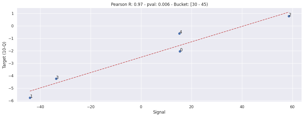
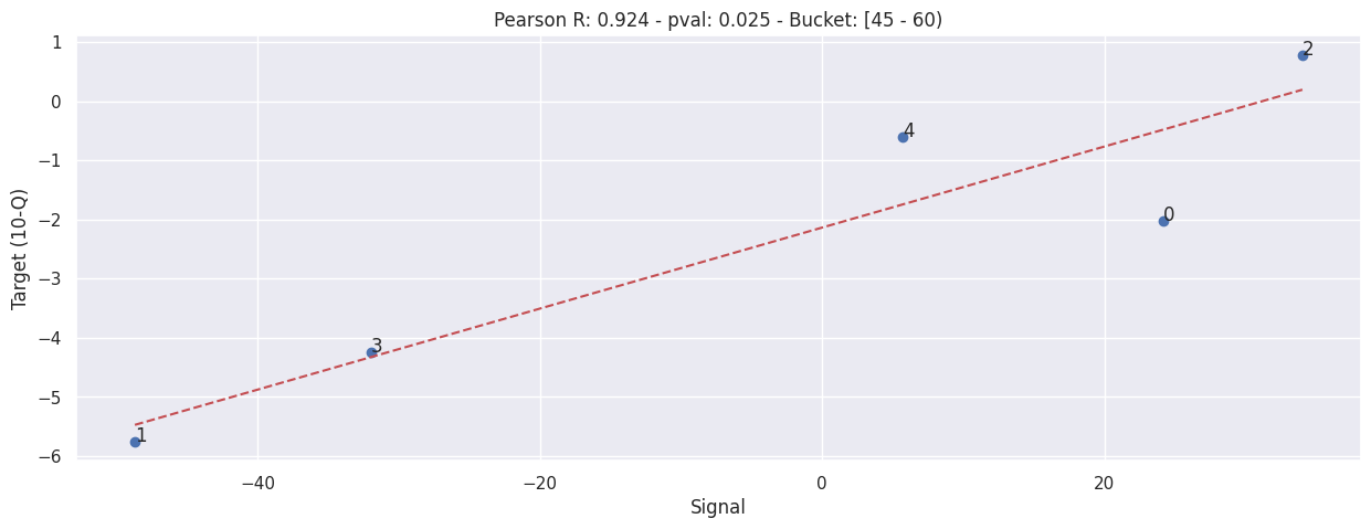
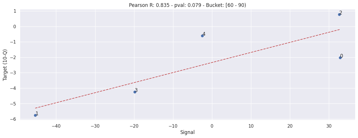
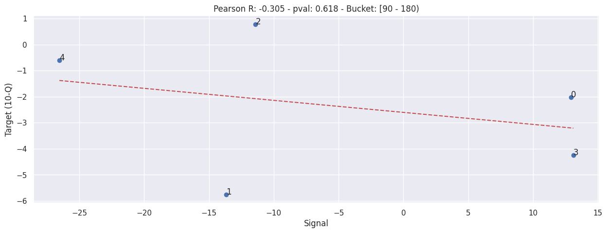
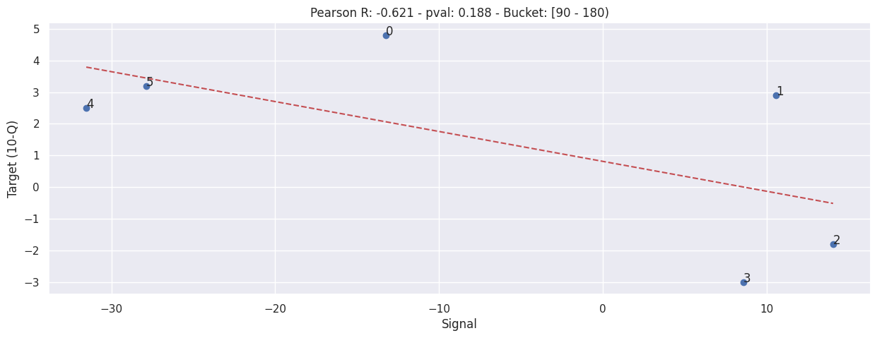
Evaluation by correlation

for bucket in ALL_BUCKETS:
    evaluate(
        SIGNALS[("waitrose", bucket)],
        TARGETS["waitrose"],
        f"Bucket: [{constants.DWELL_BUCKETS[bucket - 1]} - {constants.DWELL_BUCKETS[bucket]})",
    )

Sainsbury’s

Sainsbury’s 10Q is a bit weird for a few reasons:-

• They use a rather irregular reporting cycle, they release result for the past 16, 28, 15, 52 weeks at different times;

• They don’t report in store sales numbers directly, they release the like-for-like percentage changes instead;

• They don’t release in large store sales result in every report, only 28 weeks and 52 weeks report contains such result; (These are the values we will use, as this closer align to our signal)

Read 10Q

df_sainsburys_10q = read_10q("./data/sainsburys-supermarket-trading-statements.csv")

creating start dates from weeks

display_shrinked_dataframe(df_sainsburys_10q)

	comp_end_date	base_end_date	comp_start_date	base_start_date	comp_weeks	base_weeks	net_sales_pct_change
0	2023-03-04	2022-03-05	2022-03-05	2021-03-06	52	52	4.800000
1	2022-09-17	2021-09-18	2022-03-05	2021-03-06	28	28	2.900000
2	2022-03-05	2021-03-06	2021-03-06	2020-03-07	52	52	-1.800000
3	2021-09-18	2020-09-19	2021-03-06	2020-03-07	28	28	-3.000000
4	2021-03-06	2020-03-07	2020-03-07	2019-03-09	52	52	2.500000
5	2020-09-19	2019-09-21	2020-03-07	2019-03-09	28	28	3.200000

Sum our signal

extract_siganl_sum(df_sainsburys_10q, brand="sainsburys")

extract_signals_and_targets(df_sainsburys_10q, "sainsburys")

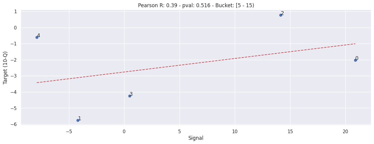
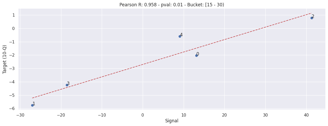
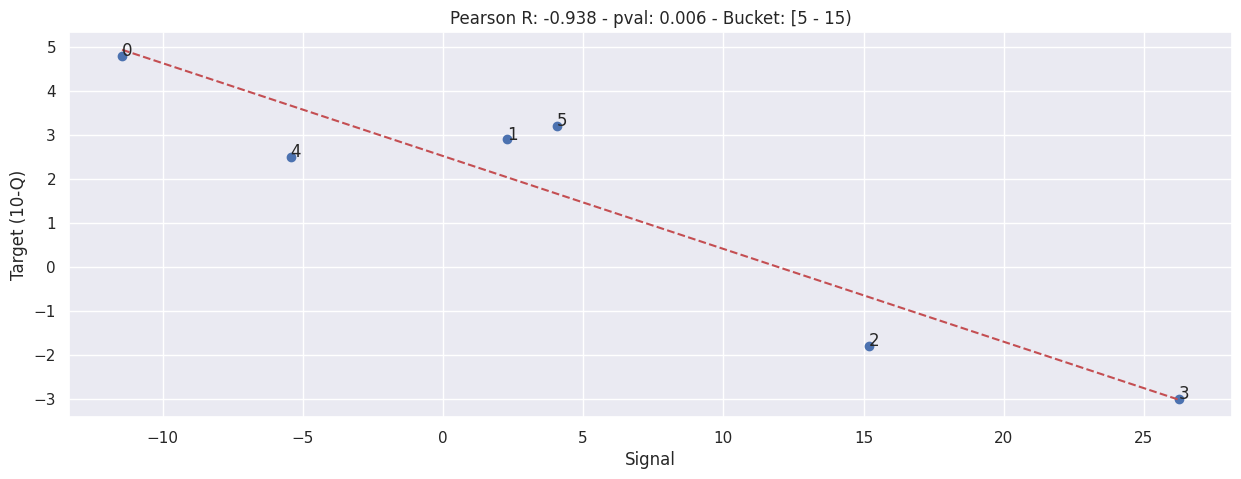
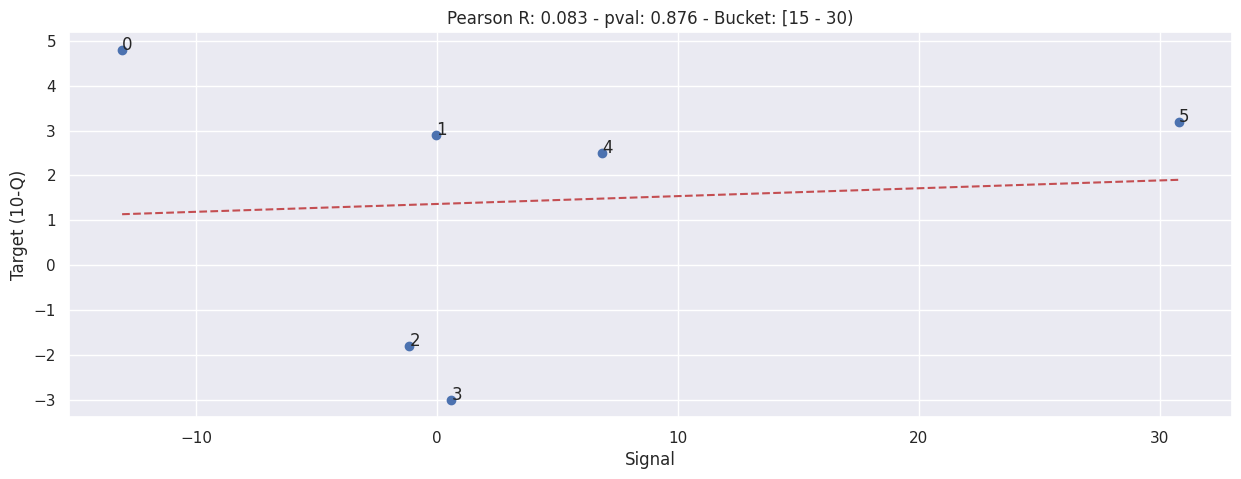
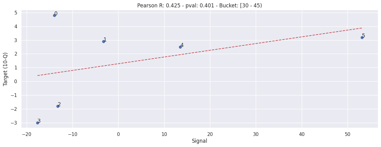
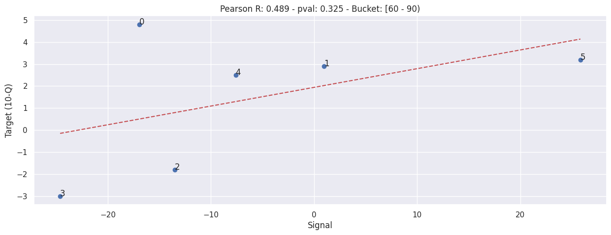
Evaluation by correlation

for bucket in ALL_BUCKETS:
    evaluate(
        SIGNALS[("sainsburys", bucket)],
        TARGETS["sainsburys"],
        f"Bucket: [{constants.DWELL_BUCKETS[bucket - 1]} - {constants.DWELL_BUCKETS[bucket]})",
    )

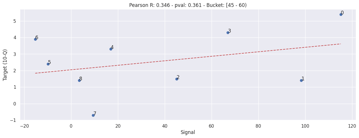
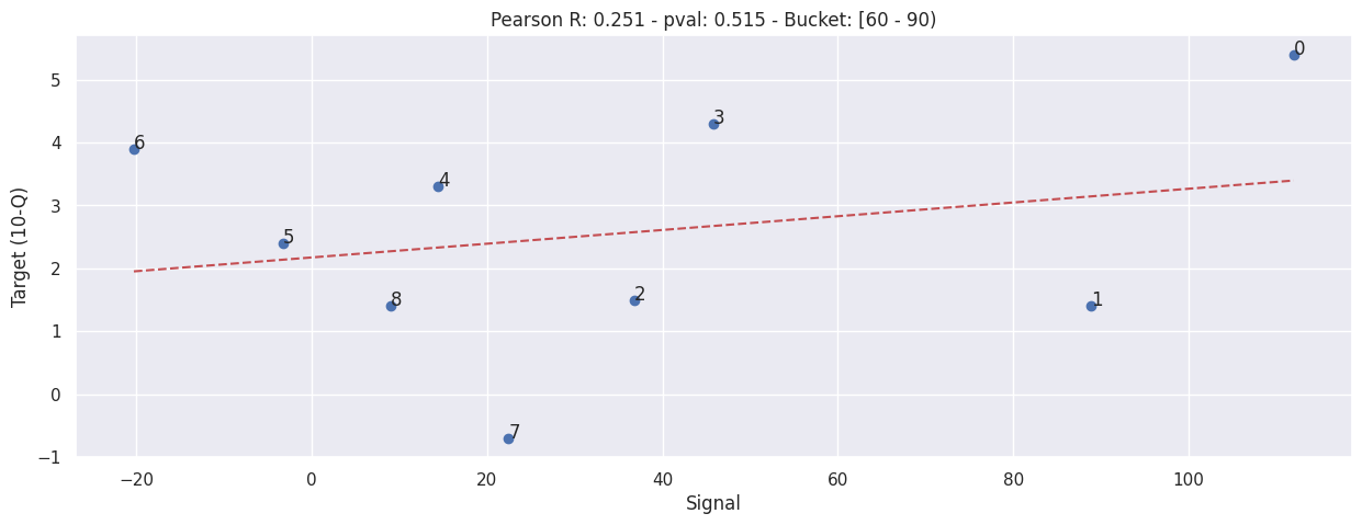
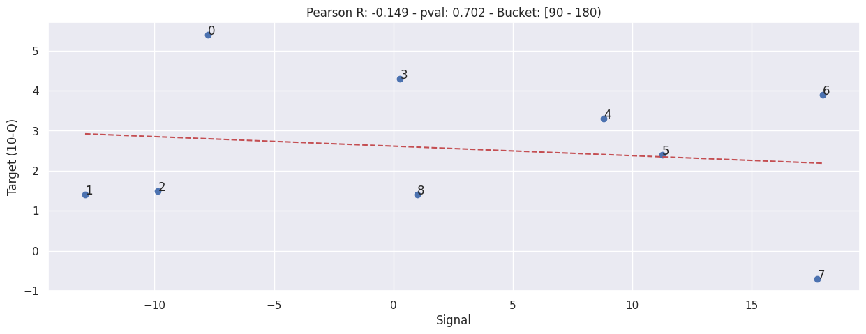
Tesco

Tesco’s 10Q is a bit weird for a few reasons (similar to Sainsbury’s):-

• They use a rather irregular reporting cycle, they release result for the past 16, 28, 15, 52 weeks at different times;

• They don’t report in store sales numbers directly, they release the like-for-like percentage changes instead;

• They don’t release in large store sales result in every report, they report these when they feel like it; (These are the values we will use, as this closer align to our signal)

Read 10Q

df_tesco_10q = read_10q("./data/tesco-trading-statements.csv")

creating start dates from weeks

display_shrinked_dataframe(df_tesco_10q)

	comp_end_date	base_end_date	comp_start_date	base_start_date	comp_weeks	base_weeks	net_sales_pct_change
0	2020-05-30	2019-05-25	2020-02-29	2019-02-23	13	13	5.400000
1	2020-08-29	2019-08-24	2020-02-29	2019-02-23	26	26	1.400000
2	2021-02-27	2020-02-29	2020-02-29	2019-03-02	52	52	1.500000
3	2021-08-28	2019-08-24	2021-02-27	2019-02-23	26	26	4.300000
4	2022-01-08	2020-01-04	2021-08-28	2019-08-24	19	19	3.300000
5	2022-01-08	2021-01-09	2021-08-28	2020-08-29	19	19	2.400000
6	2022-05-28	2020-05-30	2022-02-26	2020-02-29	13	13	3.900000
7	2022-05-28	2021-05-29	2022-02-26	2021-02-27	13	13	-0.700000
8	2022-08-27	2021-08-28	2022-02-26	2021-02-27	26	26	1.400000

Sum our signal

extract_siganl_sum(df_tesco_10q, brand="tesco")

extract_signals_and_targets(df_tesco_10q, "tesco")

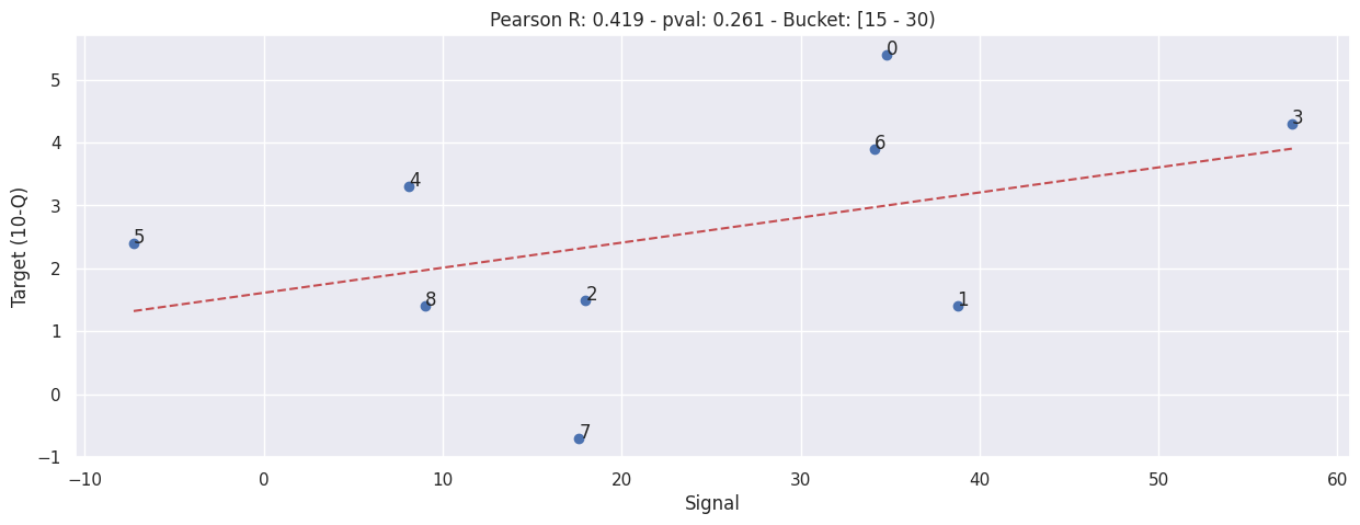
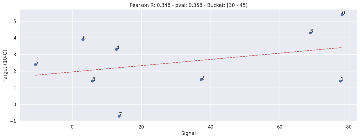
Evaluation by correlation

for bucket in ALL_BUCKETS:
    evaluate(
        SIGNALS[("tesco", bucket)],
        TARGETS["tesco"],
        f"Bucket: [{constants.DWELL_BUCKETS[bucket - 1]} - {constants.DWELL_BUCKETS[bucket]})",
    )

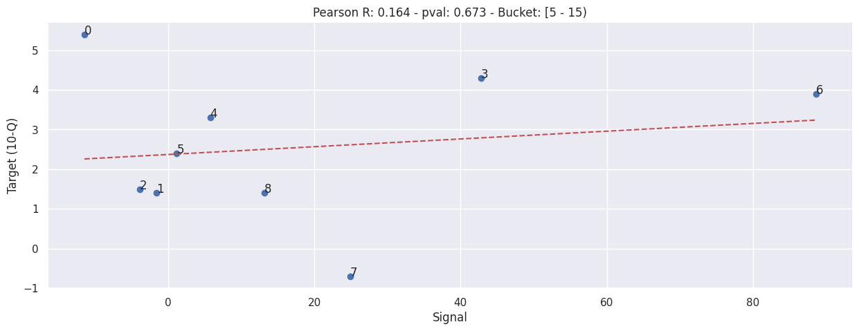
ASDA

No available data.

Morrison

No available in store sales data, there is however sales data, but given how drastic Covid-19 has changed consumer behaviour, there is no point in correlating the series as it’s just increasing noise. (More and more people are shopping online and travelling to the shop less, can’t treat proportion of online shopper as constant anymore)

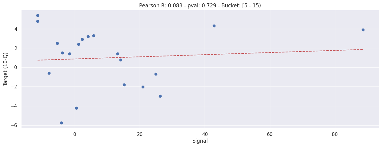
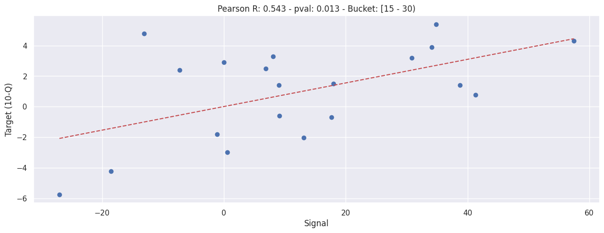
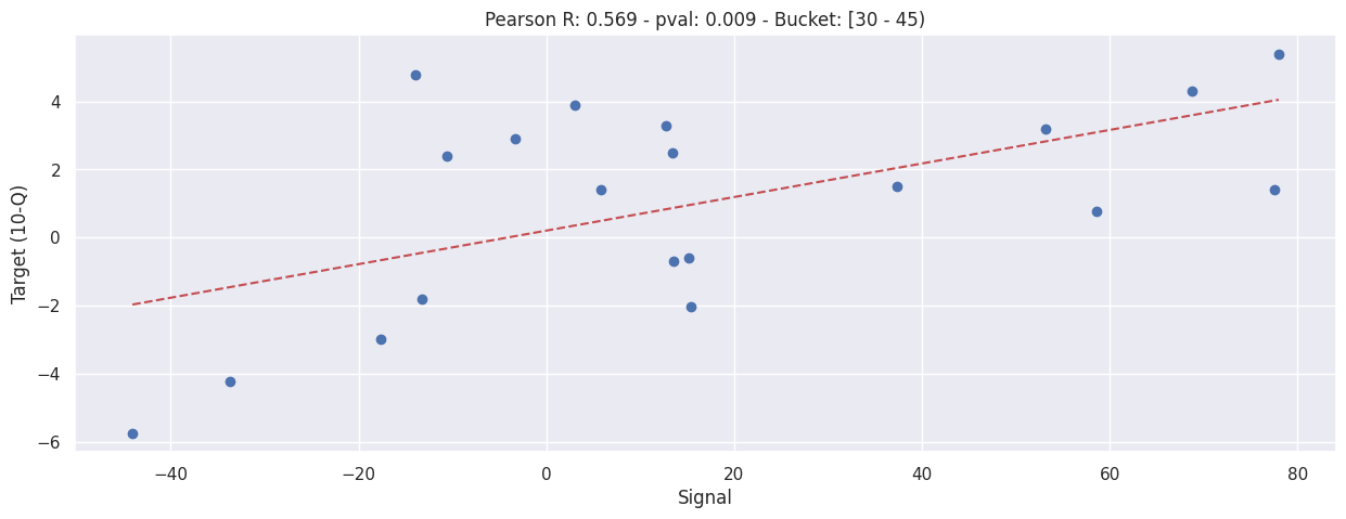
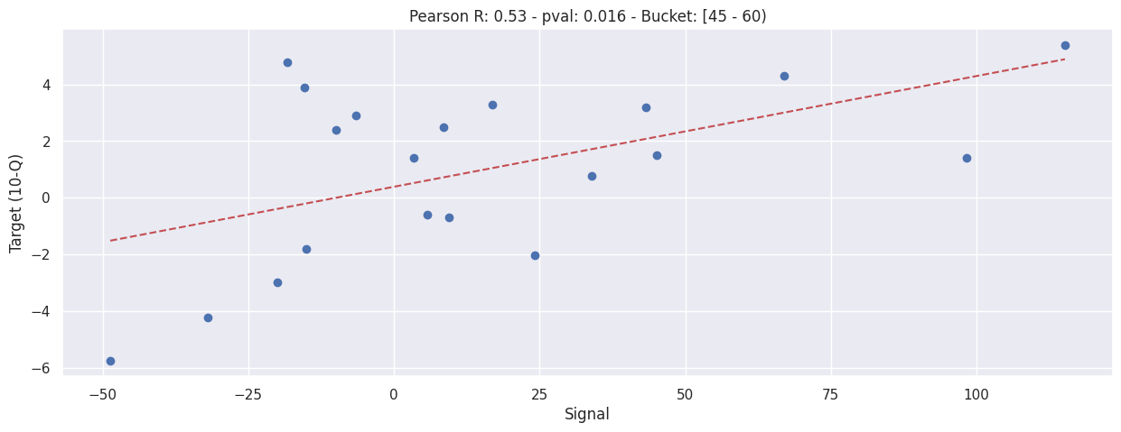
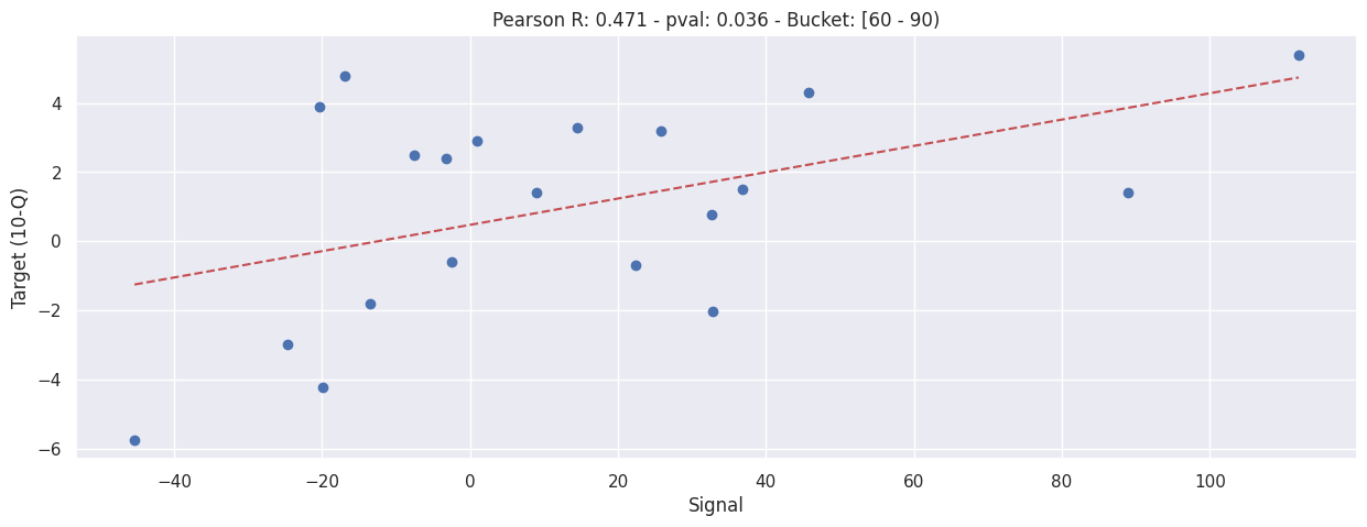
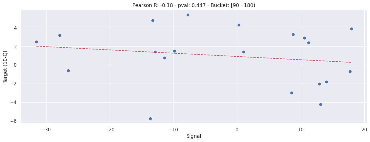
Combine Sainsbury’s, Waitrose and Tesco

for bucket in ALL_BUCKETS:
    evaluate(
        pd.concat(
            [
                value.set_axis(value.index.map(lambda x: f"{key}/{x}"))
                for key, value in SIGNALS.items()
                if key[-1] == bucket
            ]
        ),
        pd.concat(
            [
                value.set_axis(value.index.map(lambda x: f"{key}/{x}"))
                for key, value in TARGETS.items()
            ]
        ),
        f"Bucket: [{constants.DWELL_BUCKETS[bucket - 1]} - {constants.DWELL_BUCKETS[bucket]})",
    )