Time Series Plots

# Configuration and import
import pandas as pd
import matplotlib.pyplot as plt
import seaborn as sns
from IPython.display import display

sns.set_style("darkgrid")
sns.set(rc={'figure.figsize':(15, 5)})

# Read genereated signals
df = pd.concat(
    [
        pd.read_parquet("./data/output/asda.parquet"),
        pd.read_parquet("./data/output/sainsburys.parquet"),
        pd.read_parquet("./data/output/waitrose.parquet"),
        pd.read_parquet("./data/output/tesco.parquet"),
        pd.read_parquet("./data/output/morrison.parquet"),
        pd.read_parquet("./data/output/lidl.parquet"),
    ],
    axis=1,
)
# Apply rolling median to not make graph super noisy
df = df.rolling('7D').median()

# Massage data

df_unstacked = (
    df.unstack().rename("average_visit_time").reset_index(level=1).rename_axis("brand").reset_index()
)
df_market_share = (
    (df.div(df.sum(axis=1), axis=0) * 100)
    .unstack()
    .rename("market_share")
    .reset_index(level=1)
    .rename_axis("brand")
    .reset_index()
)

# Some helper plot functions
def plot_visit_time_per_capita(df):
    sns.lineplot(df, hue="brand", x="datestamp", y="average_visit_time")
    fig = plt.gcf()
    fig.autofmt_xdate(rotation=20)
    ax = plt.gca()
    ax.legend(loc="center left", bbox_to_anchor=(1, 0.5))
    plt.title("Visit time per panel capita")
    plt.ylabel("Visit time per panel capita \n (minutes per panel population)")
    plt.xlabel("Date")
    plt.ylim(0, 0.8)


def plot_market_share(df, ylim_max: int = 45):
    sns.lineplot(df, hue="brand", x="datestamp", y="market_share")
    fig = plt.gcf()
    fig.autofmt_xdate(rotation=20)
    ax = plt.gca()
    ax.legend(loc="center left", bbox_to_anchor=(1, 0.5))
    plt.title("Market share by visit time per panel capita")
    plt.ylabel("Market Share (%)")
    plt.xlabel("Date")
    plt.ylim(0, ylim_max)


def plot_market_share_pct_change(df):
    df_monthly = (
        df.groupby(
            [
                "brand",
                (
                    (
                        df["datestamp"]
                        # NOTE: Add one day if month start because month begin date offset will shift to previous
                        #       month otherwise.
                        + pd.Timedelta("1D") * df["datestamp"].dt.is_month_start
                    )
                    - pd.offsets.MonthBegin()
                ),
            ]
        )["market_share"]
        .mean()
        .reset_index()
    )

    df_monthly_market_share_merged = pd.merge(
        df_monthly.assign(cmp_datestamp=df_monthly["datestamp"].apply(lambda x: x.replace(year=x.year + 1))),
        df_monthly,
        how="inner",
        left_on=["cmp_datestamp", "brand"],
        right_on=["datestamp", "brand"],
        suffixes=("_current", "_next"),
    )

    df_monthly_market_share_merged["market_share_pct_change"] = (
        df_monthly_market_share_merged["market_share_next"]
        / df_monthly_market_share_merged["market_share_current"]
        - 1
    ) * 100

    sns.lineplot(df_monthly_market_share_merged, hue="brand", x="datestamp_next", y="market_share_pct_change")
    fig = plt.gcf()
    fig.autofmt_xdate(rotation=20)
    ax = plt.gca()
    ax.legend(loc="center left", bbox_to_anchor=(1, 0.5))
    plt.title("YoY Change of market share by visit time per panel capita")
    plt.ylabel("Market Share change (%)")
    plt.xlabel("Date")

Visit time per capita for all 6 brands

Let’s start with a simple plot of all time series.

plot_visit_time_per_capita(df_unstacked)

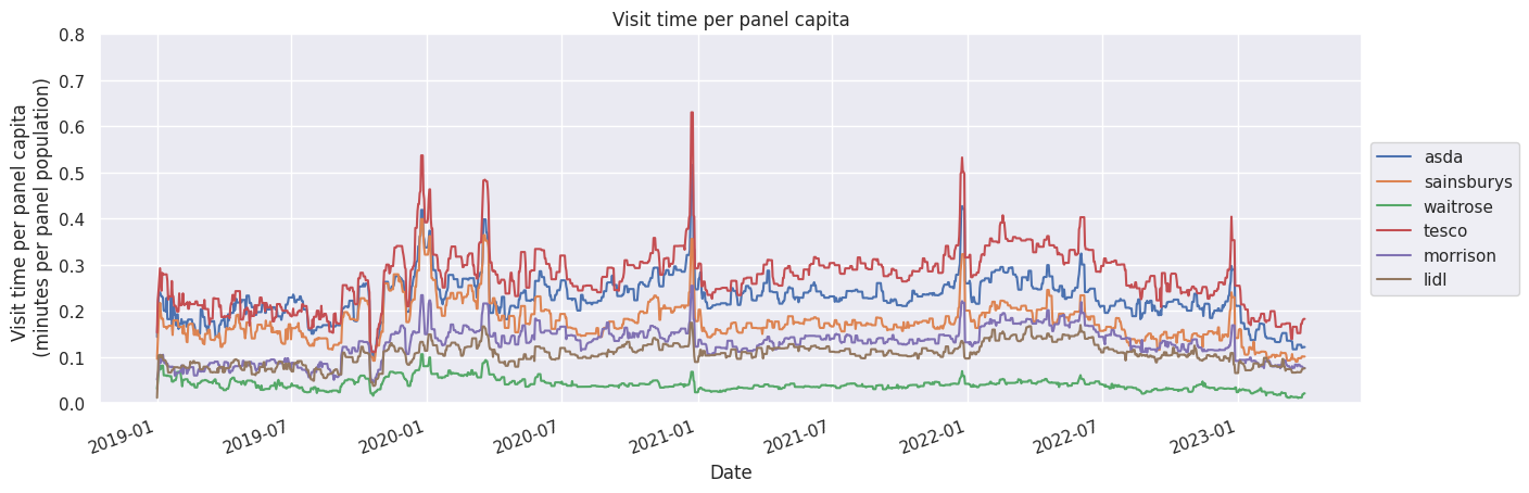
Spikes before the new year correspond to shopping behaviour prior to Christmas, this is somewhat expected.

Market share of visit time per capita for all 6 brands

To provide a better cross-sectional view of what’s going on with the same data, we divide each series with the sum of all series.

plot_market_share(df_market_share)

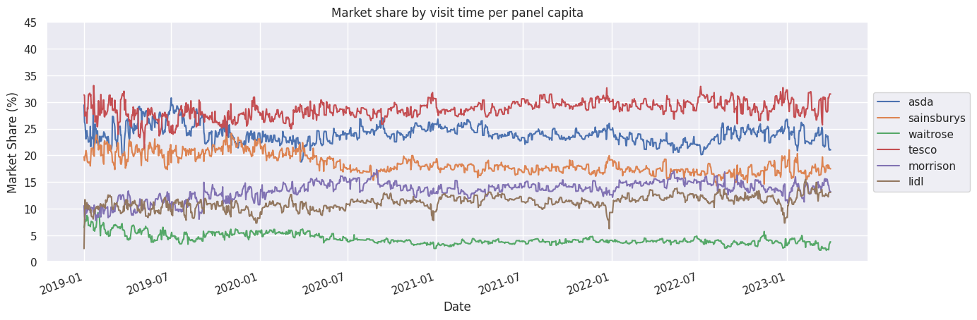
Observation 1: Spikes before the new year in the previous graph is not visibile anymore. This is a good sanity check.

Observation 2: Asda seems to be slightly higher than expected and Waitrose is slightly lower than expected.

We suspect this is because our metric is visit time per capita, instead of spend (per capita or otherwise), spend per unit time of ASDA is believed to be lower based on anecdotal experiencem, likewise, this also explains why visit time per panel capita of Waitrose seems to be lower than expected.

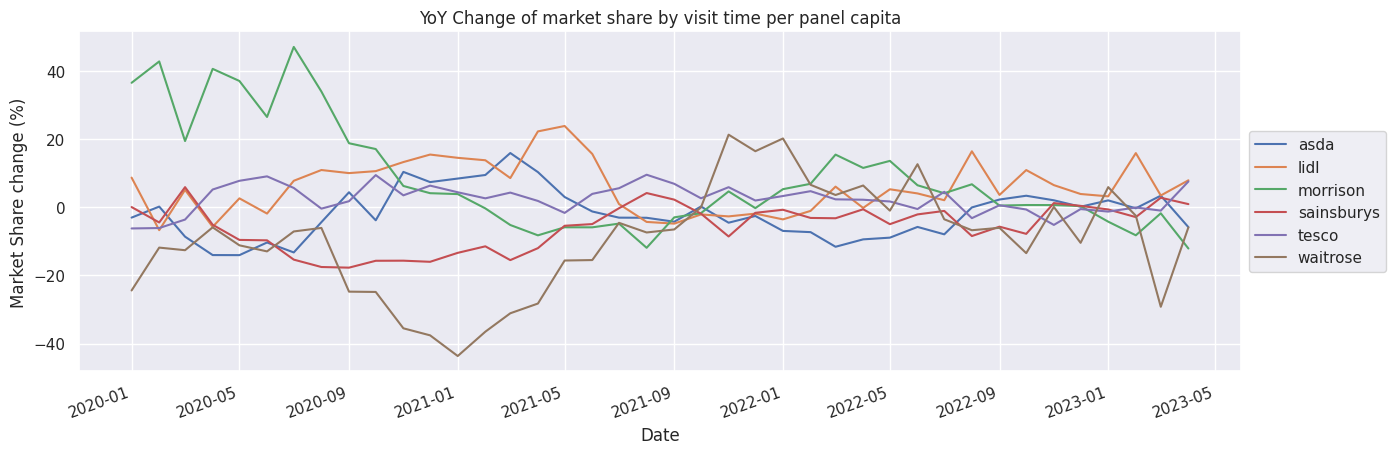
YoY change of market share of visit time per capita for all 6 brands

plot_market_share_pct_change(df_market_share)

Visit time per capita for Sainsbury’s, Tesco and Morrison

We pick the three supermarket brands that should have similar “spend per unit time” for further inspection.

# Filter for Sainsbury's, Tesco and Morrison and massage data
df_stm = df[["sainsburys", "tesco", "morrison"]]

df_stm_unstacked = (
    df_stm.unstack().rename("average_visit_time").reset_index(level=1).rename_axis("brand").reset_index()
)
df_stm_market_share = (
    (df_stm.div(df_stm.sum(axis=1), axis=0) * 100)
    .unstack()
    .rename("market_share")
    .reset_index(level=1)
    .rename_axis("brand")
    .reset_index()
)

plot_visit_time_per_capita(df_stm_unstacked)

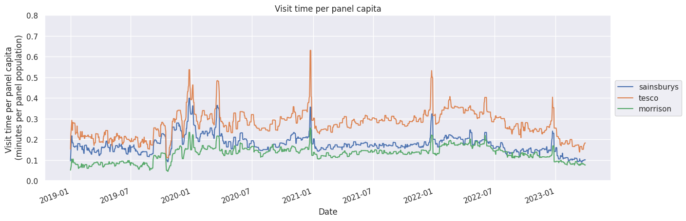
No additional remarks to be made.

Market share of visit time per capita for Sainsbury’s, Tesco and Morrison

Repeat of the cross-sectional study done above.

plot_market_share(df_stm_market_share, ylim_max=60)

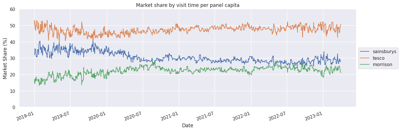
No additional remarks to be made.

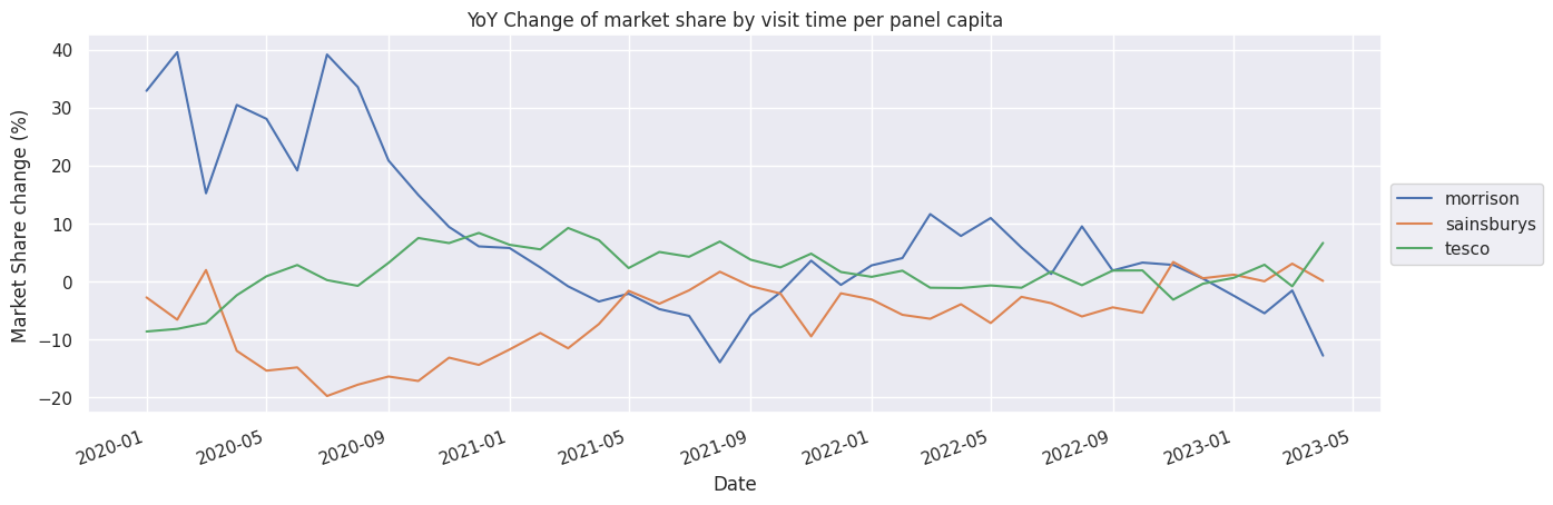
YoY change of market share of visit time per capita for Sainsbury’s, Tesco and Morrison

plot_market_share_pct_change(df_stm_market_share)